# Histogram
hist(islands)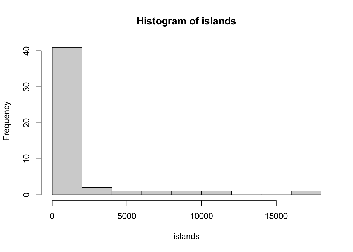

R has a number of different graphics systems. The graphics package is, by default, is installed with base R and is attached every time you start R. This package provides a lot of functionality, but it does not have a consistent syntax across different types of plots. In addition, the type of input required to construct the plot may be different for each type of plot and, in fact, the same type of plot may allow various types of input.
# Histogram
hist(islands)
# Boxplot
boxplot(islands)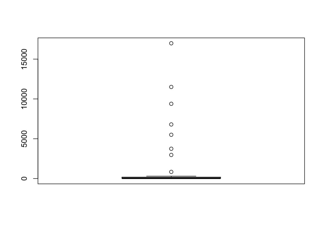
# Boxplots
boxplot(count ~ spray, data = InsectSprays)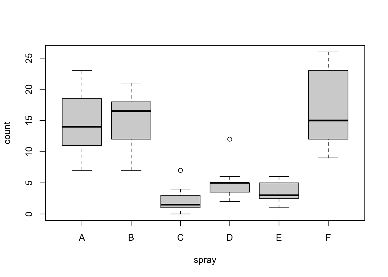
# Scatterplots
plot(x = cars$speed, y = cars$dist) # or
plot(dist ~ speed, data = cars) # using a formula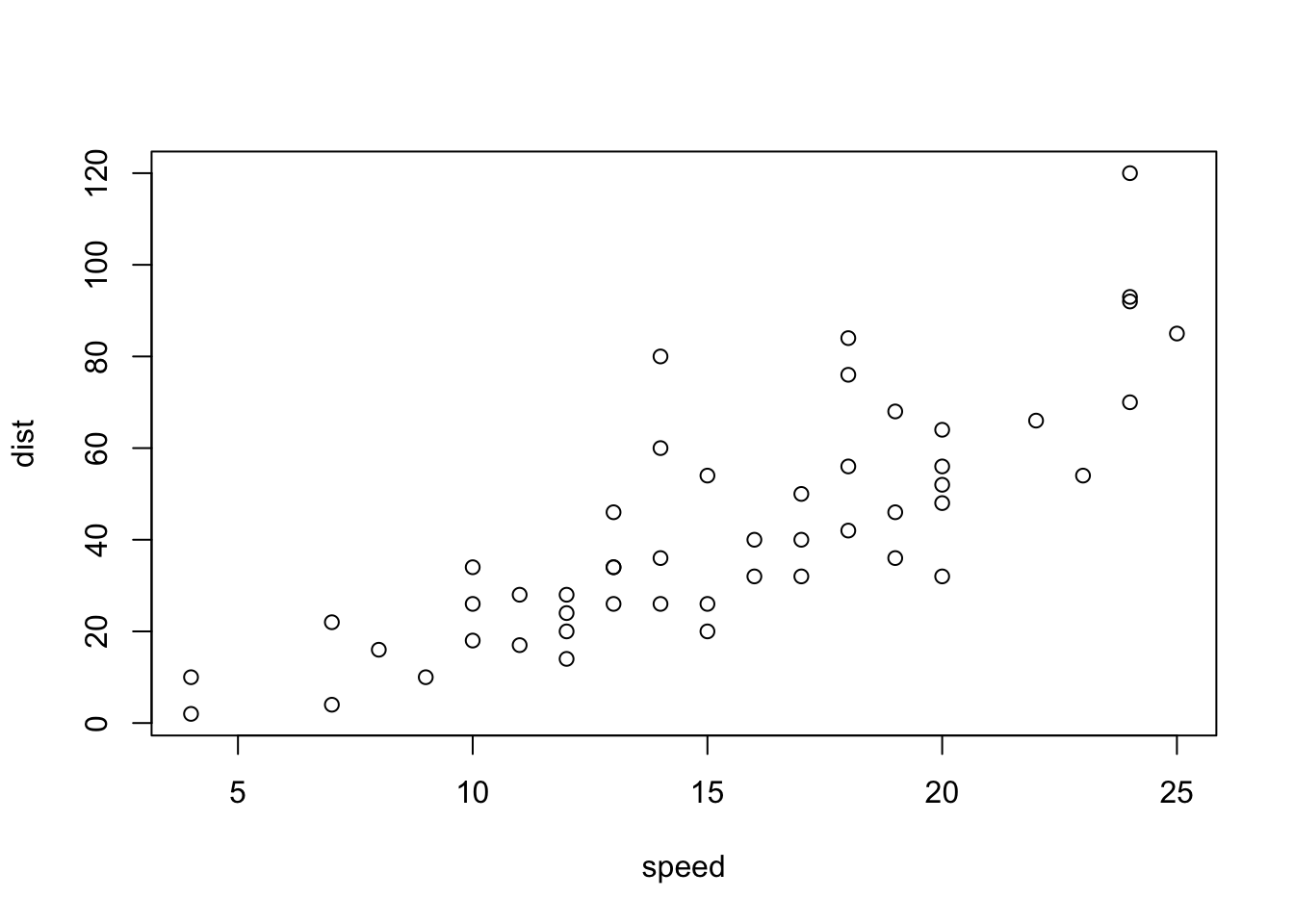
# Line plot
plot(unemploy ~ date,
     data = ggplot2::economics,
type = "l") # in a data.frame 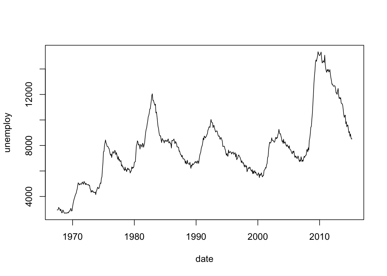
# or

plot(ggplot2::economics$date,
     ggplot2::economics$unemploy,
     type = "l") # as vectors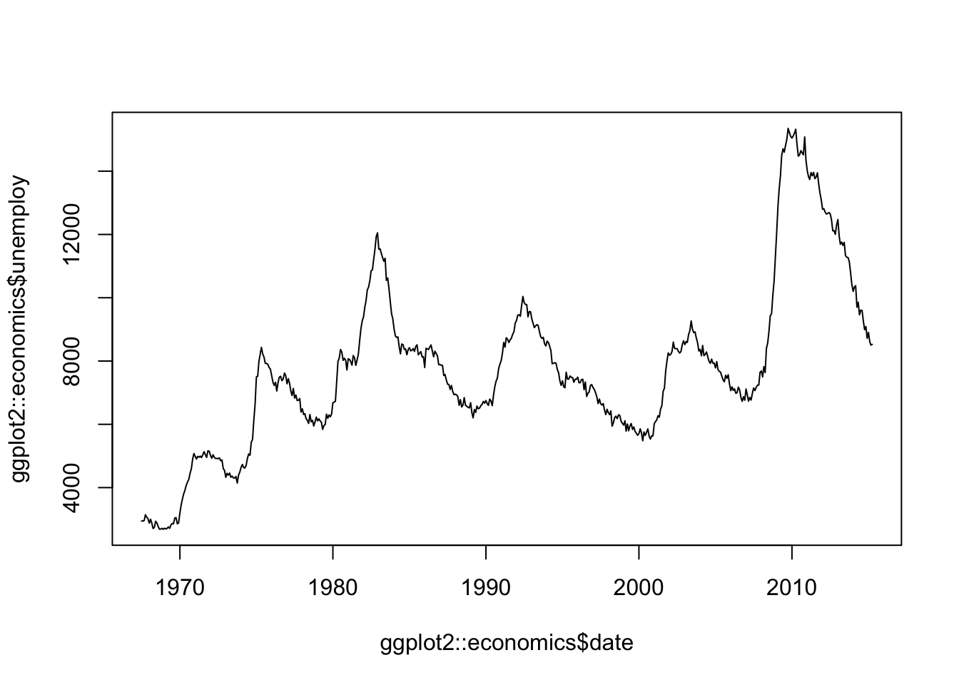
# Plot a function
curve(dnorm(x,
            mean = 3,
            sd   = 1),
      from = 0,
      to   = 6)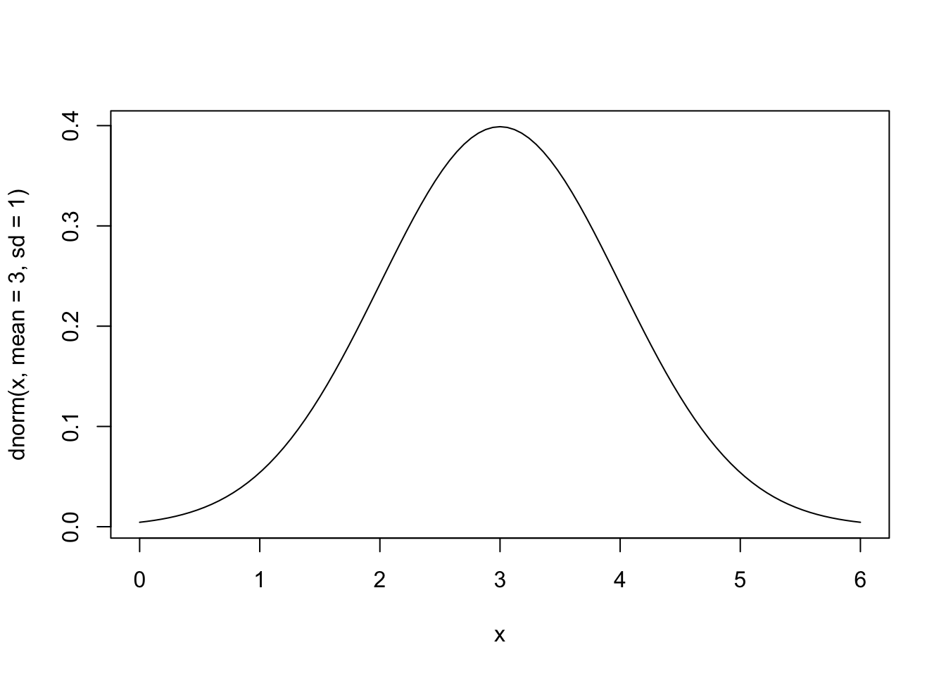
# Heatmap
image(volcano)   # notice the axes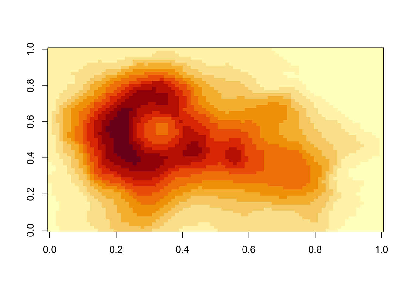
Compared to what we will see with ggplot2 graphics, base R graphics are relatively terse, i.e. the amount of code is minimal.
Using base graphics, each function uses a different data type.
# Base R graphics use all different types of data
class(islands)
[1] "numeric"class(InsectSprays)[1] "data.frame"class(cars)[1] "data.frame"class(ggplot2::economics)[1] "spec_tbl_df" "tbl_df" "tbl" "data.frame" class(volcano)[1] "matrix" "array"