14  ggplot2 intro

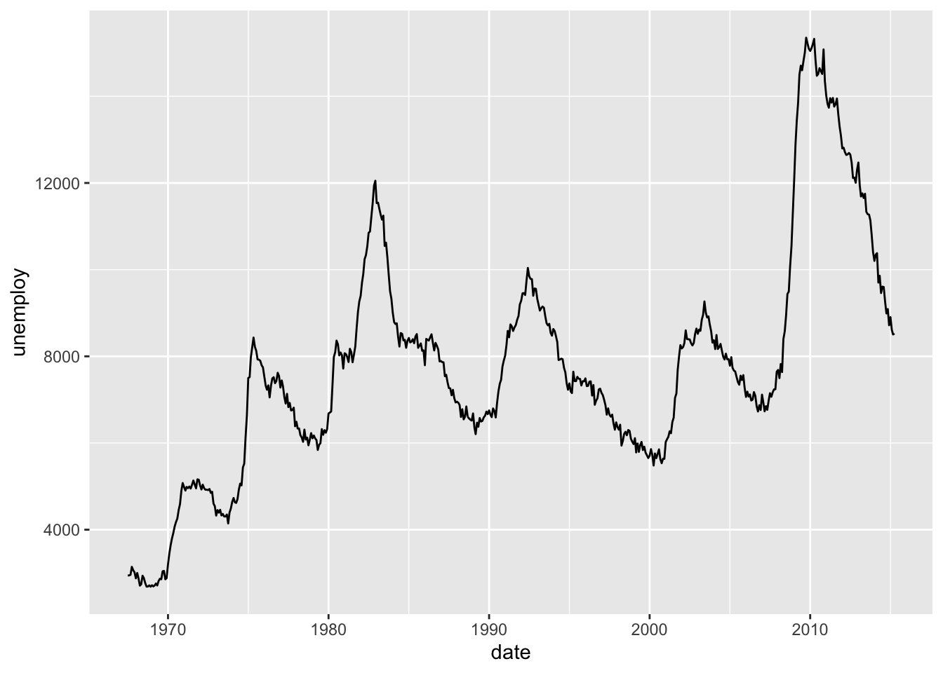
This chapter will provide a number of examples of ggplot2 graphics. ggplot2 graphics are built on the Grammar of Graphics and provide a consistent interface across different types of plots.

library("tidyverse")

── Attaching core tidyverse packages ──────────────────────── tidyverse 2.0.0 ──
✔ dplyr     1.1.4.9000     ✔ readr     2.1.5     
✔ forcats   1.0.0          ✔ stringr   1.5.1     
✔ ggplot2   3.5.2          ✔ tibble    3.3.0     
✔ lubridate 1.9.4          ✔ tidyr     1.3.1     
✔ purrr     1.0.4          
── Conflicts ────────────────────────────────────────── tidyverse_conflicts() ──
✖ dplyr::filter() masks stats::filter()
✖ dplyr::lag()    masks stats::lag()
ℹ Use the conflicted package (<http://conflicted.r-lib.org/>) to force all conflicts to become errors

14.1 Histograms

# Histogram
d <- data.frame(area = islands)
ggplot(data    = d, 
       mapping = aes(x = area)) + 
  geom_histogram()

`stat_bin()` using `bins = 30`. Pick better value with `binwidth`.

14.2 Boxplots

# Single boxplot
ggplot(data    = d, 
       mapping = aes(x = area)) + 
  geom_boxplot()

# Multiple boxplots
ggplot(data = InsectSprays, 
       mapping = aes(
         x = spray, 
         y = count)) + 
  geom_boxplot()

14.3 Scatterplot

# Scatterplot
ggplot(data = cars, 
       mapping = 
         aes(
           x = speed, 
           y = dist)) + 
  geom_point()

14.4 Line plot

# Line plot
ggplot(data = economics,
      mapping = aes(
         x = date,
         y = unemploy
       )) +
  geom_line()

14.5 Function

# Plot a function
ggplot(data    = data.frame(x = seq(0, 6)),
       mapping = aes(x = x)) + 
  
  stat_function(fun  = dnorm,
                args = list(
                  mean = 3, 
                  sd   = 1
                ))

14.6 Heatmap

# Heatmap
# Tidy the data
d <- reshape2::melt(volcano) # similar to tidyr::pivot_longer

ggplot(data = d, 
       mapping = aes(
         x    = Var1,     # Var1, Var2, and value
         y    = Var2,     # are the default names
         fill = value)) + # used by `reshape2::melt()`
  geom_raster() 

14.7 Summary

As a general rule, working with ggplot2 graphics will require a bit more data wrangling to get the data into the appropriate tidy (long) format. Once the data is in the correct format, construction of each plot uses a similar syntax:

• provide the name of the data frame,
• provide the mapping of the visual aesthetics of the plots, and
• provide the type of plot desired.