We will start with loading up the necessary packages using the library() command.
library("tidyverse") # for read_csv
── Attaching core tidyverse packages ──────────────────────── tidyverse 2.0.0 ──
✔ dplyr     1.1.4.9000     ✔ readr     2.1.5
✔ forcats   1.0.0          ✔ stringr   1.5.1
✔ ggplot2   3.5.2          ✔ tibble    3.3.0
✔ lubridate 1.9.4          ✔ tidyr     1.3.1
✔ purrr     1.0.4
── Conflicts ────────────────────────────────────────── tidyverse_conflicts() ──
✖ dplyr::filter() masks stats::filter()
✖ dplyr::lag()    masks stats::lag()
ℹ Use the conflicted package (<http://conflicted.r-lib.org/>) to force all conflicts to become errors
In this chapter, we will introduce how you can read data files into R. Ultimately, the code will look like
d <-read_csv("ToothGrowth.csv")
Before, we can start reading data in from our file system, we need to 1) understand the concept of a working directory and 2) have a file that we can read.
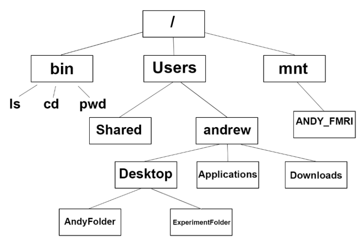
27.1 File system
The figure below shows an example directory structure based on a Mac (or Linux) system.
You can set the working directory in RStudio by going to
Session > Set Working Directory > Choose Working Directory
Alternatively, we can use the setwd() function.
# Set the current working directory?setwd
Use RStudio projects!! This will set your working directory to the same folder every time you open that project.
27.1.3 Absolute path
An absolute path will work no matter what your current working directory is
d <- readr::read_csv("~/Downloads/example.csv") # ~ is home directoryd <- readr::read_csv("/Users/niemi/Downloads/example.csv")
While absolute paths are convenient I highly recommend you don’t use them because their use create scripts that are not reproducible. The scripts won’t work correctly for you on any other system. The scripts won’t work for somebody else on their system.
27.1.4 Relative path
A relative path is evaluated relative to the current working directory. To move up a directory, use “..”. To move down a directory, use the name of the directory.
d <- readr::read_csv("data/example.csv")d <- readr::read_csv("../data/example.csv")d <- readr::read_csv("../../example.csv")
In order to use relative paths, you need to know what directory is expected to be the current working directory when running a script. I often put this information in the metadata of the file.
## Execute this script from its directory## OR## Execute this script from the project directory#
The former is convenient because you always know where the script should be executed (as long as nobody moves the file). The latter is convenient because all scripts can be executed from the same folder and thus, when you are working within a project, you do not need to constantly change your working directory. A downside is that it is not always obvious what the project directory is. In the large projects I have been part of, the latter is typical.
27.2 File interaction
27.2.1 Write
Before we try to read a csv file, we need to make sure there is a csv file available to be read. We will accomplish this by writing a csv file to the current working directory.
We will discuss more about writing a csv file when discussing exporting data.
27.2.2 Read
To read in a csv file you can use the read_csv function in the readr package.
# Read a csv filed <-read_csv("ToothGrowth.csv")
Rows: 60 Columns: 3
── Column specification ────────────────────────────────────────────────────────
Delimiter: ","
chr (1): supp
dbl (2): len, dose

ℹ Use `spec()` to retrieve the full column specification for this data.
ℹ Specify the column types or set `show_col_types = FALSE` to quiet this message.
      len            supp                dose
 Min.   : 4.20   Length:60          Min.   :0.500
 1st Qu.:13.07   Class :character   1st Qu.:0.500
 Median :19.25   Mode  :character   Median :1.000
 Mean   :18.81                      Mean   :1.167
 3rd Qu.:25.27                      3rd Qu.:2.000
 Max.   :33.90                      Max.   :2.000
Generally, a csv file will contain commas (or semi-colons) that separate the columns in the data and the same number of columns in every row. The file should also have a header row, immediately preceding the first data row, that provides the names for each of the columns. Optionally, the file could contain additional metadata above the header row.
Some (Canvas….ahem!) add additional row(s) between the header and the data. This should not be done as it makes it difficult for standard software, including R, to read the file since data is assumed to immediately come after the header.
If you want to include additional rows, you can include rows above the header row. The skip argument of read_csv() can be used to skip rows before the header row.
27.3.2 Excel
We can utilize R to read directly from Excel files. If you would like to try, you can use the readxl package and the read_excel() function within that package.
install.packages("readxl")?readxl::read_excel
While reading directly from Excel files can work, it may be easier to “Save as…” the Excel sheet into a CSV file and then read that CSV file.
Generally, I don’t suggest storing data in binary formats, but these formats can be useful to store intermediate data. For example, if there is some important results from a statistical analysis that takes a long time to perform (I’m looking at you Bayesians) you might want to store the results in a binary format.
27.3.4.1 RData
There are two functions that will save RData files: save() and save.image(). The latter will save everything in the environment while the former will only save what it is specifically told to save. Both of these are read using the load() function.
a <-1save(a, file ="a.RData")
Remember, we do NOT want to load .RData files by default. But, we my want to intentionally load these files with the load() function.
rm(a) # make sure the a object does not existload("a.RData") # retains the object names
27.3.4.2 RDS
An RDS file contains a single R object. These files can be written using saveRDS() and read using readRDS().
saveRDS(a, file ="a.RDS")rm(a)
When you read this file, you need to save the result into an R object.
b <-readRDS("a.RDS")
27.4 Cleanup
If you have followed along with the code in this chapter, you will have a few extraneous files around. To remove these files use the following code.