42 Logistic Regression

Author

Jarad Niemi

library("tidyverse"); theme_set(theme_bw())

── Attaching core tidyverse packages ──────────────────────── tidyverse 2.0.0 ──
✔ dplyr     1.1.4.9000     ✔ readr     2.1.5     
✔ forcats   1.0.0          ✔ stringr   1.5.1     
✔ ggplot2   4.0.0          ✔ tibble    3.3.0     
✔ lubridate 1.9.4          ✔ tidyr     1.3.1     
✔ purrr     1.0.4          
── Conflicts ────────────────────────────────────────── tidyverse_conflicts() ──
✖ dplyr::filter() masks stats::filter()
✖ dplyr::lag()    masks stats::lag()
ℹ Use the conflicted package (<http://conflicted.r-lib.org/>) to force all conflicts to become errors

library("gridExtra")


Attaching package: 'gridExtra'

The following object is masked from 'package:dplyr':

    combine

library("Sleuth3")

Logistic regression can be used when your response variable is a count with a known maximum. Similar to regression, explanatory variables can be continuous, categorical, or both. Here we will consider models up to two explanatory variables.

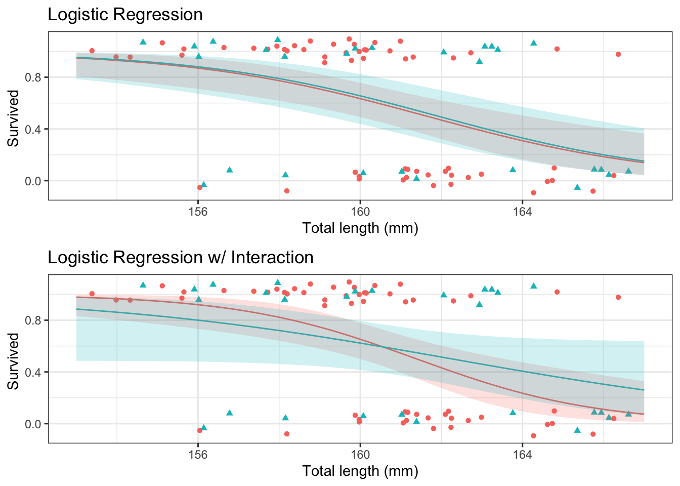
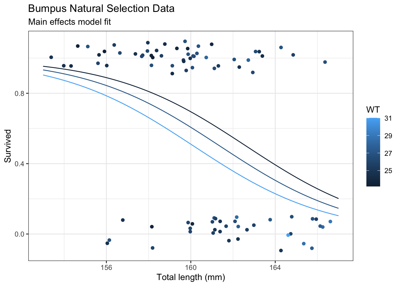
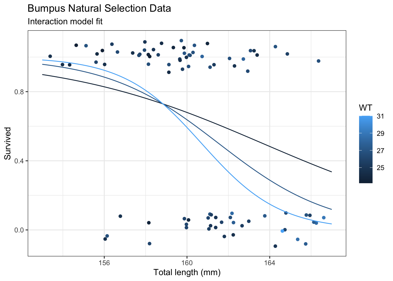
When there are two (or more) explanatory variables, we can consider a main effects model or models with interactions. The main effects model will result in parallel lines or line segments while the interaction model will result in more flexible lines or line segments. These lines will be straight when plotting the response variable on a logistic axis, although we will rarely do so since the interpretation is very difficult.

42.1 Model

Let \(Y_i\) be the number of successes out of \(n_i\) attempts. The logistic regression model assumes Assume \[ Y_i \stackrel{ind}{\sim} Bin(n_i, p_i), \quad \mbox{logit}(p_i) = \log\left(\frac{p_i}{1-p_i} \right) = \beta_0 + \beta_1X_{i,1} + \cdots + \beta_{p} X_{i,p} \] where \(Bin\) designates a binomial random variable and, for observation \(i\),

\(p_i\) is the probability of success
\(p_i/(1-p_i)\) is the odds, and
\(\log[p_i/(1-p_i)]\) is the log-odds.

A common special case of this model is when \(n_i=1\) for all \(i\). In this situation, the response is binary since \(Y_i\) can only be 0 or 1.

42.1.1 Assumptions

The assumptions in a logistic regression are

observations are independent
observations have a binomial distribution (each with its own mean)

and

the relationship between the probability of success and the explanatory variables is through the \(\mbox{logit}\) function.

Later we will need the inverse of the logit function. We will call this expit.

# Inverse of logit function
expit <- function(x) {
  1 / (1 + exp(-x))
}

We will create another function to round probabilities to 2 decimal places

# Function to keep a fixed number of decimal places
keep_decimals <- function(x, decimals = 2) {
  # Check if input is numeric
  if (!is.numeric(x)) stop("Input must be numeric")
  
  # Format with fixed decimal places
  formatted <- format(round(x, decimals), nsmall = decimals)
  
  return(formatted)
}

42.1.2 Interpretation

When no interactions are in the model, an exponentiated regression coefficient is the multiplicative effect on the odds for a 1 unit change in the explanatory variable when all other explanatory variables are help constant. Mathematically, we can see this through \[ \frac{p'}{1-p'} = e^{\beta_j} \times \frac{p}{1-p} \] where \(p\) is the probability when \(X_j = x\) and \(p'\) is the probability when \(X_j = x+1\). If the \(X_j\) are categorical, then this is the effect of being in the category versus the reference category.

If \(\beta_j\) is positive, then \(e^{\beta_j} > 1\) and the probability goes up. If \(\beta_j\) is negative, then \(e^{\beta_j} < 0\) and the probability goes down.

42.1.3 Inference

Individual regression coefficients are evaluated using \(z\)-statistics derived from the Central Limit Theorem and data asymptotics. This approach is known as a Wald test. Similarly confidence intervals and prediction intervals are constructed using the same assumptions and are thus referred to as Wald intervals.

Collections of regression coefficients are evaluated with drop-in-deviance where the residual deviances from the model with and without these terms in the model are compared with a \(\chi^2\)-test.

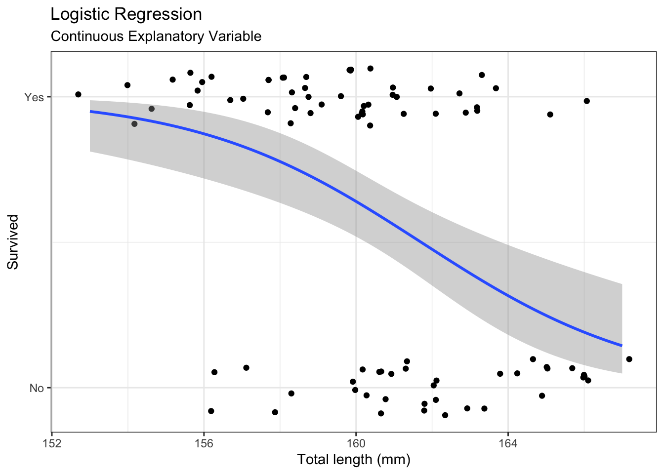
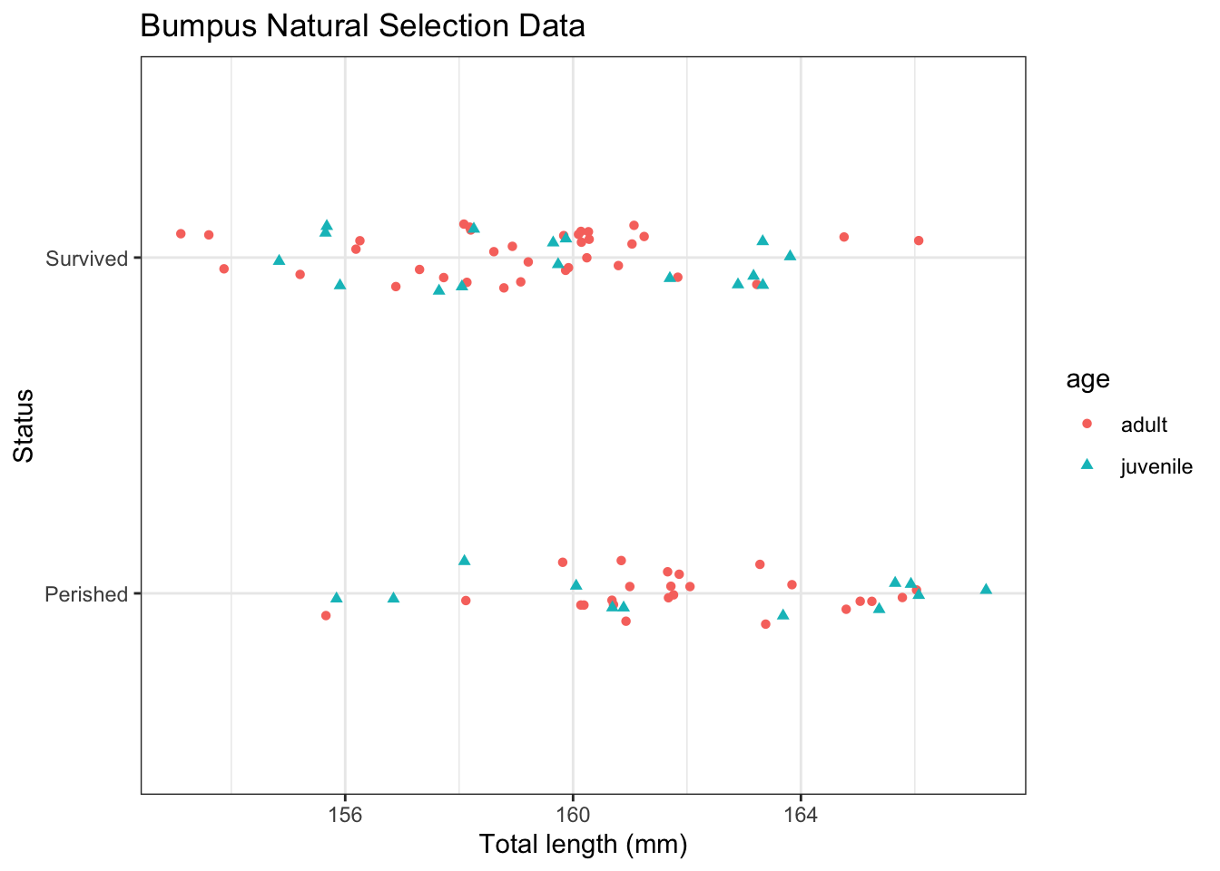
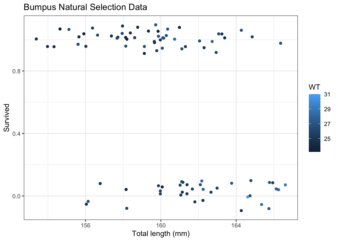
42.2 Continuous variable

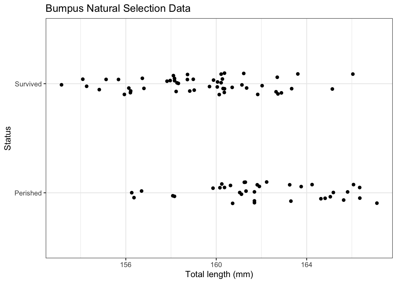
First we will consider simple logistic regression where there is a single continuous explanatory variable.

# ex2016
ggplot(ex2016,
       aes(x = TL,
           y = Status)) +
  labs(
    x     = "Total length (mm)",
    title = "Bumpus Natural Selection Data"
  ) + 
  geom_jitter(height = 0.1)

An alternative plot would count the number of observations and use these counts as the size of the points.

# Summarize the data
d <- ex2016 |>
  group_by(TL, Status) |>
  summarize(
    n = n()
  )

`summarise()` has grouped output by 'TL'. You can override using the `.groups`
argument.

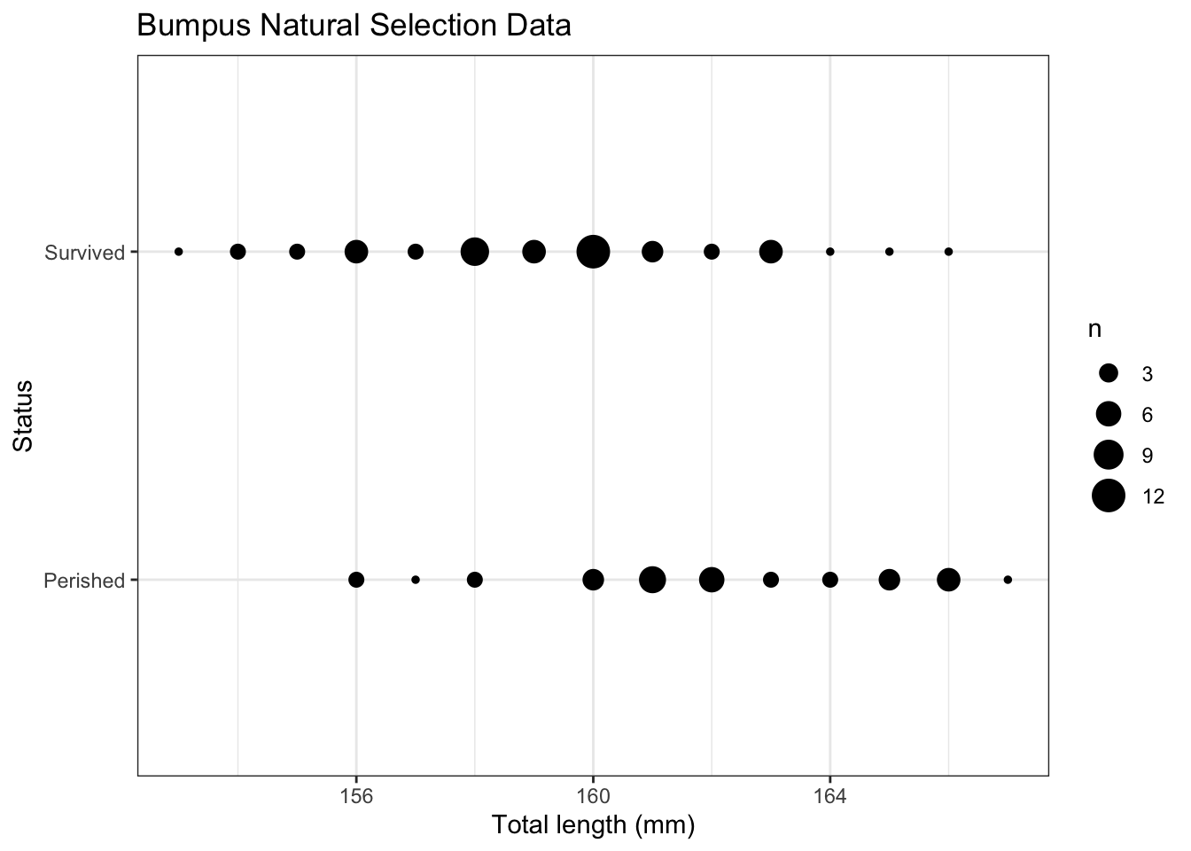
g <- ggplot(d,
       aes(x = TL,
           y = Status)) +
  labs(
    x     = "Total length (mm)",
    title = "Bumpus Natural Selection Data"
  ) +
  geom_point(
    aes(size = n)) 

g

When running a logistic regression, you need to decide what success is. This choice is arbitrary, but important to how you interpret the regression. It is a good practice to be explicit about what is success by a numerical vector where 1 represents success and 0 represents failure. Here we will define surviving as success.

# Fit logistic regression when response is binary
m <- glm(as.numeric(Status == "Survived") ~ # 0 = Perished, 1 = Survived
           TL,                              # Explanatory variable(s)
         data   = ex2016,
         family = "binomial")

# Summary
summary(m)


Call:
glm(formula = as.numeric(Status == "Survived") ~ TL, family = "binomial", 
    data = ex2016)

Coefficients:
            Estimate Std. Error z value Pr(>|z|)    
(Intercept) 54.49312   14.57866   3.738 0.000186 ***
TL          -0.33698    0.09062  -3.719 0.000200 ***
---
Signif. codes:  0 '***' 0.001 '**' 0.01 '*' 0.05 '.' 0.1 ' ' 1

(Dispersion parameter for binomial family taken to be 1)

    Null deviance: 118.008  on 86  degrees of freedom
Residual deviance:  99.788  on 85  degrees of freedom
AIC: 103.79

Number of Fisher Scoring iterations: 4

# Coefficients 
m$coefficients

(Intercept)          TL 
 54.4931246  -0.3369782

# Confidence interval
exp(confint(m)[2,]) # multiplicative effect on the odds

Waiting for profiling to be done...

    2.5 %    97.5 % 
0.5880293 0.8419684

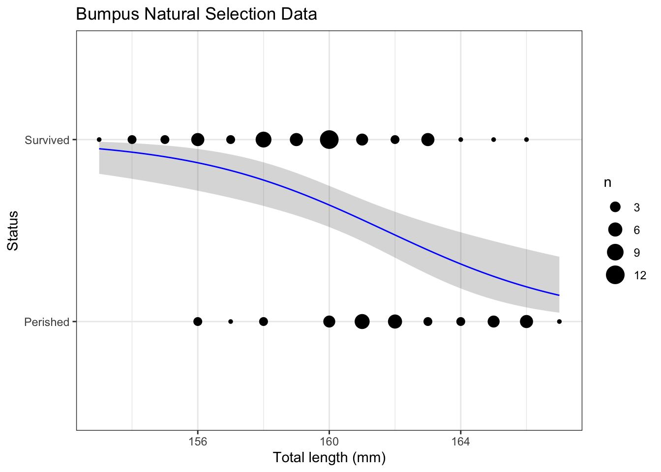
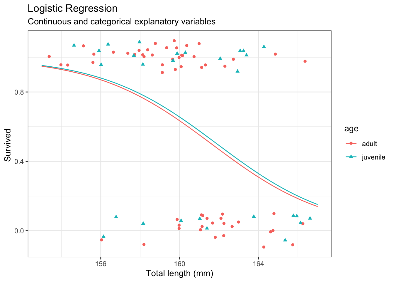
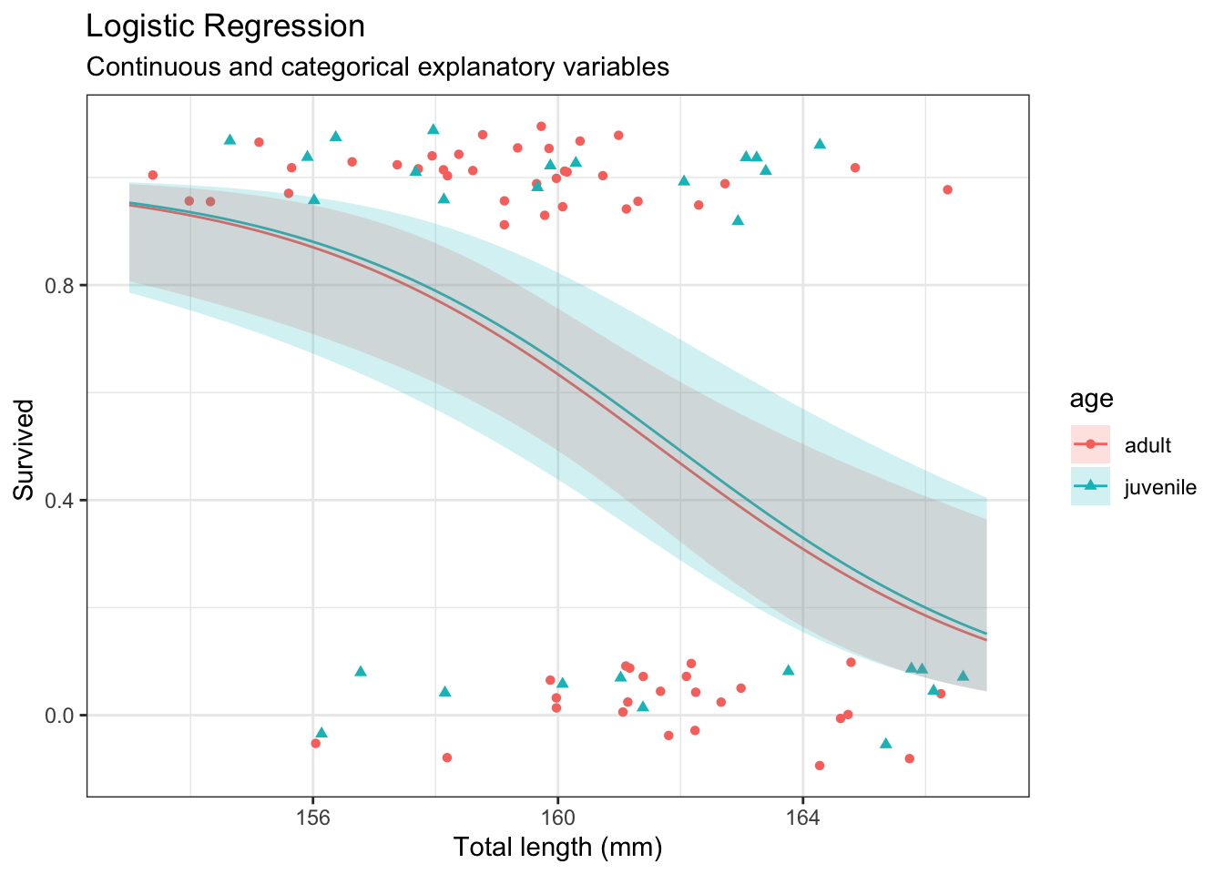
To construct

# Create new data
nd <- data.frame(
  TL = seq(
    from   = min(ex2016$TL),
    to     = max(ex2016$TL),
    length = 101
  )
)

# Create predictions and combine with data
p <-  
  bind_cols(
    nd, 
    
    predict(m,             
            newdata = nd, 
            se.fit  = TRUE) |>
      as.data.frame() |>
      
      # Manually construct confidence intervals
      mutate(
        lwr = fit - qnorm(0.975) * se.fit,
        upr = fit + qnorm(0.975) * se.fit,
        
        # Expit to get to probability scale
        # also + 1 so line is within two levels because Perished is 1 and Survived is 2
        Status = expit(fit) + 1,
        lwr    = expit(lwr) + 1,
        upr    = expit(upr) + 1
      ) 
  )

# Plot
pg <- g + 
  geom_ribbon(
    data = p,
    mapping = aes(
      ymin = lwr,
      ymax = upr
    ),
    alpha = 0.2
  ) +
  geom_line(
    data = p,
    color = "blue"
  ) 

pg

42.2.1 Grouped data

# Group data
dg <- d |>
  pivot_wider(id_cols     = TL,
              names_from  = Status,
              values_from = n,
              values_fill = 0) |> # make NAs 0
  arrange(TL)

To fit the logistic regression with grouped data, we need a matrix where the first column is the successes and the second column is the failures.

# Fit logistic regression with grouped data
m2 <- glm(cbind(Survived,    # Successes 
                Perished) ~  # Failures
            TL,              # Explanatory variable(s)
          data = dg,
          family = "binomial")

The two approaches will result in the same answers.

# Coefficients are the same
m $coefficients

(Intercept)          TL 
 54.4931246  -0.3369782

m2$coefficients

(Intercept)          TL 
 54.4931246  -0.3369782

# Confindence intervals are the same
confint(m )

Waiting for profiling to be done...

                 2.5 %     97.5 %
(Intercept) 27.9645127 85.7107597
TL          -0.5309786 -0.1720128

confint(m2)

Waiting for profiling to be done...

                 2.5 %     97.5 %
(Intercept) 27.9645124 85.7107595
TL          -0.5309786 -0.1720128

42.2.2 geom_smooth()

To use geom_smooth(), you need to construct a numeric binary variable (0-1).

# Create binary variable
d <- ex2016 |>
  mutate(
    survived = Status == "Survived",
    survived = as.numeric(survived) # 0 = no failure, 1 = failure
  )

# Create plot using binary variable
ggplot(d,
       aes(
         x = TL, 
         y = survived
       )) +
  geom_jitter(
    height = 0.1
  ) + 
  geom_smooth( 
    method      = 'glm', 
    method.args = list(family = 'binomial')) +
  
  scale_y_continuous(
    breaks = c(0, 1),
    labels = c("No","Yes")
  ) +
  labs(
    x        = "Total length (mm)",
    y        = 'Survived',
    title    = "Logistic Regression",
    subtitle = "Continuous Explanatory Variable"
  )

`geom_smooth()` using formula = 'y ~ x'

42.3 Categorical variable

Logistic regression can be used with categorical variables. When both the explanatory variable and response variable are discrete, the data are easily represented in a table.

# Create interpretable variables
d <- ex2016 |>
  mutate(
    age   = ifelse(AG == 1, "adult",   "juvenile"),
    small = ifelse(TL < 160, "small", "not small")   # this is used later
  )

# Show results in a table
d |>
  group_by(age) |>
  summarize(
    n = n(),
    p = keep_decimals(sum(Status == "Survived")/n)
  )

# A tibble: 2 × 3
  age          n p    
  <chr>    <int> <chr>
1 adult       59 0.59 
2 juvenile    28 0.57

Fit logistic regression model using a categorical explanatory variable.

# Fit Logistic regression model
m <- glm(as.numeric(Status == "Survived") ~ age,
         data   = d,
         family = 'binomial')

# Model summary
summary(m)


Call:
glm(formula = as.numeric(Status == "Survived") ~ age, family = "binomial", 
    data = d)

Coefficients:
            Estimate Std. Error z value Pr(>|z|)
(Intercept)  0.37729    0.26502   1.424    0.155
agejuvenile -0.08961    0.46483  -0.193    0.847

(Dispersion parameter for binomial family taken to be 1)

    Null deviance: 118.01  on 86  degrees of freedom
Residual deviance: 117.97  on 85  degrees of freedom
AIC: 121.97

Number of Fisher Scoring iterations: 4

# Confidence intervals
exp(confint(m)[2,]) # CI for multiplicative effect on the odds (juvenile vs. adult)

Waiting for profiling to be done...

    2.5 %    97.5 % 
0.3679314 2.3018519

Calculate predictions

# Create data frame with unique explanatory variable values
nd <- d |>
  select(age) |>
  unique()

# Predict
p <- bind_cols(
  nd,
  predict(m,
          newdata = nd,
          se.fit = TRUE)|>
      as.data.frame() |>
      
      # Manually construct confidence intervals
      mutate(
        lwr = fit - qnorm(0.975) * se.fit,
        upr = fit + qnorm(0.975) * se.fit,
        
        # Expit to get to probability scale
        Status  = expit(fit),
        lwr     = expit(lwr),
        upr     = expit(upr)
      ) 
  )

p |> 
  mutate(p   = keep_decimals(Status),
         lwr = keep_decimals(lwr),
         upr = keep_decimals(upr)) |>
  select(age, p, lwr, upr)

        age    p  lwr  upr
1     adult 0.59 0.46 0.71
60 juvenile 0.57 0.39 0.74

42.4 Two categorical variables

Logistic regression can be used with two categorical variables.

# Data frame for table
t <- d |>
  group_by(age, small) |>
  summarize(
    n = n(),
    p = sum(Status == "Survived")/n, # survived is 'success'
    p = keep_decimals(p),
      
    .groups = "drop"
  ) 

t

# A tibble: 4 × 4
  age      small         n p    
  <chr>    <chr>     <int> <chr>
1 adult    not small    39 0.44 
2 adult    small        20 0.90 
3 juvenile not small    18 0.50 
4 juvenile small        10 0.70

t |>
  select(-n) |>
  pivot_wider(
    id_cols     = age,
    names_from  = small,
    values_from = p
  )

# A tibble: 2 × 3
  age      `not small` small
  <chr>    <chr>       <chr>
1 adult    0.44        0.90 
2 juvenile 0.50        0.70

A logistic regression model works linearly on the link scale.

42.4.1 Main effects

Fit main effects regression model

# Fit main effects logistic regression model
m <- glm(as.numeric(Status == "Survived") ~ age + small,
         data   = d,
         family = 'binomial')

# Model summary
summary(m)


Call:
glm(formula = as.numeric(Status == "Survived") ~ age + small, 
    family = "binomial", data = d)

Coefficients:
            Estimate Std. Error z value Pr(>|z|)   
(Intercept)  -0.1330     0.3088  -0.431  0.66664   
agejuvenile  -0.1364     0.5007  -0.272  0.78524   
smallsmall    1.7893     0.5580   3.207  0.00134 **
---
Signif. codes:  0 '***' 0.001 '**' 0.01 '*' 0.05 '.' 0.1 ' ' 1

(Dispersion parameter for binomial family taken to be 1)

    Null deviance: 118.01  on 86  degrees of freedom
Residual deviance: 105.54  on 84  degrees of freedom
AIC: 111.54

Number of Fisher Scoring iterations: 3

# Confidence intervals
exp(confint(m)[2:3,]) # multiplicative effect on the odds

Waiting for profiling to be done...

                2.5 %    97.5 %
agejuvenile 0.3244291  2.345813
smallsmall  2.1392233 19.766716

Calculate predictions

# Create data frame with unique explanatory variable values
nd <- d |>
  select(age, small) |>
  unique()

# Predict
p <- bind_cols(
  nd,
  predict(m,
          newdata = nd,
          se.fit = TRUE)|>
      as.data.frame() |>
      
      # Manually construct confidence intervals
      mutate(
        lwr = fit - qnorm(0.975) * se.fit,
        upr = fit + qnorm(0.975) * se.fit,
        
        # Expit to get to probability scale
        Status = expit(fit), 
        lwr    = expit(lwr),
        upr    = expit(upr)
      ) 
  )

p |> 
  mutate(p   = keep_decimals(Status),
         lwr = keep_decimals(lwr),
         upr = keep_decimals(upr)) |>
  select(age, small, p, lwr, upr)

        age     small    p  lwr  upr
1     adult     small 0.84 0.65 0.94
2     adult not small 0.47 0.32 0.62
60 juvenile     small 0.82 0.59 0.94
62 juvenile not small 0.43 0.25 0.64

Construct table to provide predictions.

# Rearrange prediction table
p |> 
  mutate(
    estimate_with_ci = 
      paste0(keep_decimals(Status, 2),
            " (", keep_decimals(lwr, 2), ", ",
                 keep_decimals(upr, 2), ")")
  ) |>
  select(-fit, -se.fit, -residual.scale,
         -lwr, -upr, -Status) |>
  pivot_wider(
    id_cols     = age,
    names_from  = small,
    values_from = estimate_with_ci
  )

# A tibble: 2 × 3
  age      small             `not small`      
  <chr>    <chr>             <chr>            
1 adult    0.84 (0.65, 0.94) 0.47 (0.32, 0.62)
2 juvenile 0.82 (0.59, 0.94) 0.43 (0.25, 0.64)

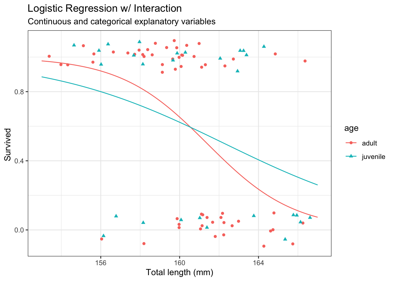
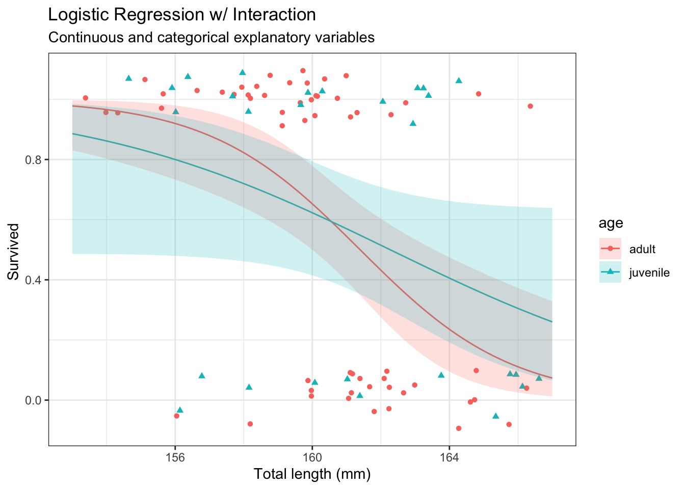
42.4.2 Interaction

Fit interaction regression model

# Fit main effects Poisson regression model
m <- glm(as.numeric(Status == "Survived") ~ age * small,
         data   = d,
         family = 'binomial')

# Model summary
summary(m)


Call:
glm(formula = as.numeric(Status == "Survived") ~ age * small, 
    family = "binomial", data = d)

Coefficients:
                       Estimate Std. Error z value Pr(>|z|)   
(Intercept)             -0.2578     0.3229  -0.798  0.42462   
agejuvenile              0.2578     0.5714   0.451  0.65183   
smallsmall               2.4551     0.8122   3.023  0.00251 **
agejuvenile:smallsmall  -1.6078     1.1654  -1.380  0.16772   
---
Signif. codes:  0 '***' 0.001 '**' 0.01 '*' 0.05 '.' 0.1 ' ' 1

(Dispersion parameter for binomial family taken to be 1)

    Null deviance: 118.01  on 86  degrees of freedom
Residual deviance: 103.60  on 83  degrees of freedom
AIC: 111.6

Number of Fisher Scoring iterations: 4

Calculate predictions

# Predict
p <- bind_cols(
  nd,
  predict(m,
          newdata = nd,
          se.fit = TRUE)|>
      as.data.frame() |>
      
      # Manually construct confidence intervals
      mutate(
        lwr = fit - qnorm(0.975) * se.fit,
        upr = fit + qnorm(0.975) * se.fit,
        
        # Expit to get to probability scale
        Status = expit(fit),
        lwr    = expit(lwr),
        upr    = expit(upr)
      ) 
  )

p |> 
  mutate(p   = keep_decimals(Status),
         lwr = keep_decimals(lwr),
         upr = keep_decimals(upr)) |>
  select(age, small, p, lwr, upr)

        age     small    p  lwr  upr
1     adult     small 0.90 0.68 0.97
2     adult not small 0.44 0.29 0.59
60 juvenile     small 0.70 0.38 0.90
62 juvenile not small 0.50 0.28 0.72

Construct table for predictions and uncertainty.

# Rearrange prediction table
p |> 
  mutate(
    estimate_with_ci = 
      paste0(keep_decimals(Status, 2),
            " (", keep_decimals(lwr, 2), ", ",
                 keep_decimals(upr, 2), ")")
  ) |>
  
  pivot_wider(
    id_cols     = age,
    names_from  = small,
    values_from = estimate_with_ci
  )

# A tibble: 2 × 3
  age      small             `not small`      
  <chr>    <chr>             <chr>            
1 adult    0.90 (0.68, 0.97) 0.44 (0.29, 0.59)
2 juvenile 0.70 (0.38, 0.90) 0.50 (0.28, 0.72)

42.5 Continuous and categorical variable

# Plot data
ggplot(d, 
       aes(
         x     = TL,
         y     = Status,
         color = age,
         shape = age
       )) +
  labs(
    x = "Total length (mm)",
    title = "Bumpus Natural Selection Data"
  ) +
  geom_jitter(height = 0.1)

42.5.1 Main effects

Fit main effects model

# Fit model
m <- glm(as.numeric(Status == "Survived") ~ age + TL,
         data     = d,
         family   = 'binomial')

# Model summary
summary(m)


Call:
glm(formula = as.numeric(Status == "Survived") ~ age + TL, family = "binomial", 
    data = d)

Coefficients:
            Estimate Std. Error z value Pr(>|z|)    
(Intercept) 54.70322   14.65061   3.734 0.000189 ***
agejuvenile  0.09494    0.53054   0.179 0.857977    
TL          -0.33846    0.09116  -3.713 0.000205 ***
---
Signif. codes:  0 '***' 0.001 '**' 0.01 '*' 0.05 '.' 0.1 ' ' 1

(Dispersion parameter for binomial family taken to be 1)

    Null deviance: 118.008  on 86  degrees of freedom
Residual deviance:  99.755  on 84  degrees of freedom
AIC: 105.76

Number of Fisher Scoring iterations: 4

# Confidence intervals
exp(confint(m)[2:3,]) # multiplicative effect on the odds

Waiting for profiling to be done...

                2.5 %    97.5 %
agejuvenile 0.3912053 3.1928321
TL          0.5863327 0.8414248

# Create prediction data frame
nd <- expand.grid(
  age = unique(d$age),
  TL = seq(
    from   = min(d$TL),
    to     = max(d$TL),
    length = 101
  )
)

# Predictions
p <- bind_cols(
  nd,
  predict(m,
          newdata = nd,
          se.fit = TRUE)|>
      as.data.frame() |>
      
      # Manually construct confidence intervals
      mutate(
        lwr = fit - qnorm(0.975) * se.fit,
        upr = fit + qnorm(0.975) * se.fit,
        
        # Expit to get to probability scale
        Status = expit(fit),
        lwr    = expit(lwr),
        upr    = expit(upr)
      ) 
  )

Plot model predictions

# Construct plot to show model predictions
g <- ggplot(d,
       aes(
         x     = TL,
         y     = as.numeric(Status == "Survived"),
         color = age,
         shape = age
       )) +
  labs(
    x = "Total length (mm)",
    title = "Bumpus Natural Selection Data"
  ) +
  geom_point(
    position = position_jitter(
      height = 0.1,
      seed = 20040328 # make jitter is reproducible
    )) 

# Add main effects regression line
gm <- g +
  geom_line(
    data = p,
    mapping = aes(
      y = Status
    )
  ) +
  labs(
    y        = "Survived ",
    x        = "Total length (mm)",
    title    = "Logistic Regression",
    subtitle = "Continuous and categorical explanatory variables"
  )

gm

# Add uncertainty
g1 <- gm + geom_ribbon(
  data = p,
  mapping = aes(
    y    = Status,
    ymin = lwr,
    ymax = upr,
    fill = age
  ),
  color = NA,
  alpha = 0.2
)

g1

42.5.2 Interaction

Fit regression model with interaction

# Fit model
m <- glm(as.numeric(Status == "Survived") ~ age * TL,
         data     = d,
         family   = 'binomial')

# Model summary
summary(m)


Call:
glm(formula = as.numeric(Status == "Survived") ~ age * TL, family = "binomial", 
    data = d)

Coefficients:
               Estimate Std. Error z value Pr(>|z|)   
(Intercept)     72.9666    22.4918   3.244  0.00118 **
agejuvenile    -37.1036    29.8885  -1.241  0.21446   
TL              -0.4521     0.1399  -3.231  0.00123 **
agejuvenile:TL   0.2311     0.1857   1.244  0.21339   
---
Signif. codes:  0 '***' 0.001 '**' 0.01 '*' 0.05 '.' 0.1 ' ' 1

(Dispersion parameter for binomial family taken to be 1)

    Null deviance: 118.008  on 86  degrees of freedom
Residual deviance:  98.173  on 83  degrees of freedom
AIC: 106.17

Number of Fisher Scoring iterations: 4

# Drop-in-deviance test
anova(m, test = "Chi")

Analysis of Deviance Table

Model: binomial, link: logit

Response: as.numeric(Status == "Survived")

Terms added sequentially (first to last)

       Df Deviance Resid. Df Resid. Dev  Pr(>Chi)    
NULL                      86    118.008              
age     1   0.0371        85    117.971    0.8472    
TL      1  18.2159        84     99.755 1.972e-05 ***
age:TL  1   1.5829        83     98.173    0.2083    
---
Signif. codes:  0 '***' 0.001 '**' 0.01 '*' 0.05 '.' 0.1 ' ' 1

# Predictions
p <- bind_cols(
  nd,
  predict(m,
          newdata = nd,
          se.fit = TRUE)|>
      as.data.frame() |>
      
      # Manually construct confidence intervals
      mutate(
        lwr = fit - qnorm(0.975) * se.fit,
        upr = fit + qnorm(0.975) * se.fit,
        
        # Expit to get to probability scale
        Status = expit(fit),
        lwr    = expit(lwr),
        upr    = expit(upr)
      ) 
  )

Plot model predictions

# Construct plot to show model predictions
gi <- g +
  geom_line(
    data = p,
    mapping = aes(
      y = Status
    )
  ) +
  labs(
    y        = "Survived ",
    x        = "Total length (mm)",
    title    = "Logistic Regression w/ Interaction",
    subtitle = "Continuous and categorical explanatory variables"
  )

gi

# Add uncertainty
g2 <- gi + geom_ribbon(
  data = p,
  mapping = aes(
    y    = Status,
    ymin = lwr,
    ymax = upr,
    fill = age
  ),
  color = NA,
  alpha = 0.2
)

g2

Put both plots in same figure.

gridExtra::grid.arrange(g1 + 
                          theme(legend.position = "none") +
                          labs(subtitle = NULL), 
                        g2 + 
                          theme(legend.position = "none") +
                          labs(subtitle = NULL), 
                        ncol = 1)

You can also use geom_smooth() which will fit the interaction model.

# Use geom_smooth()
ggplot(d,
       aes(
         x = TL,
         y = as.numeric(Status == "Survived"),
         color = age,
         shape = age
       )) +
  geom_point(
    position = position_jitter(
      height = 0.1,
      seed   = 20040328
    )
  ) +
  geom_smooth(
    method = "glm",
    method.args = list(family = 'binomial'),
    fullrange = TRUE
  ) +
  labs(
    y        = "Survived ",
    x        = "Total length (mm)",
    title    = "Logistic Regression",
    subtitle = "with geom_smooth()"
  )

`geom_smooth()` using formula = 'y ~ x'

42.6 Two continuous variables

Now we will consider two continuous explanatory variables.

# Plot
g <- ggplot(ex2016,
       aes(
         x     = TL,
         y     = as.numeric(Status == "Survived"),
         color = WT
       )) +
  geom_point(
    position = position_jitter(
      height = 0.1,
      seed   = 20040328)
  ) +
  labs(
    y     = "Survived",
    x     = "Total length (mm)",
    title = "Bumpus Natural Selection Data"
  )

g

42.6.1 Main effects

Fit regression model

# Main effects model
m <- glm(as.numeric(Status == "Survived") ~ TL + WT,
         data   = ex2016,
         family = 'binomial')

# Summary
summary(m)


Call:
glm(formula = as.numeric(Status == "Survived") ~ TL + WT, family = "binomial", 
    data = ex2016)

Coefficients:
            Estimate Std. Error z value Pr(>|z|)    
(Intercept)  53.3898    14.7203   3.627 0.000287 ***
TL           -0.3140     0.1012  -3.105 0.001906 ** 
WT           -0.1000     0.2050  -0.488 0.625567    
---
Signif. codes:  0 '***' 0.001 '**' 0.01 '*' 0.05 '.' 0.1 ' ' 1

(Dispersion parameter for binomial family taken to be 1)

    Null deviance: 118.008  on 86  degrees of freedom
Residual deviance:  99.546  on 84  degrees of freedom
AIC: 105.55

Number of Fisher Scoring iterations: 4

# Confidence intervals
exp(confint(m)[2:3,]) # CI for multiplicative effect on the odds

Waiting for profiling to be done...

       2.5 %    97.5 %
TL 0.5896227 0.8800215
WT 0.5966969 1.3432631

When both explanatory variables are continuous, select certain value of the non-x-axis variable to make lines for.

# Create prediction data frame
nd <- expand.grid(
  WT = seq(
    from   = min(ex2016$WT),
    to     = max(ex2016$WT),
    length = 3),             # limit the number of lines drawn
  TL = seq(
    from   = min(ex2016$TL),
    to     = max(ex2016$TL),
    length = 101)
)

# Predictions
p <- bind_cols(
  nd,
  predict(m,
          newdata = nd,
          se.fit = TRUE)|>
      as.data.frame() |>
      
      # Manually construct confidence intervals
      mutate(
        lwr = fit - qnorm(0.975) * se.fit,
        upr = fit + qnorm(0.975) * se.fit,
        
        # Expit to get to probability scale
        Status = expit(fit),
        lwr    = expit(lwr),
        upr    = expit(upr)
      ) 
  )

Plot model predictions

# Plot predictions
pg <- g + 
  geom_line(
    data = p,
    mapping = aes(
      y     = Status,
      group = WT
    )) +
  labs(
    subtitle = "Main effects model fit"
  )

pg

42.6.2 Interaction

Fit regression model

# Main effects model
m <- glm(as.numeric(Status == "Survived") ~ TL * WT,
         data   = ex2016,
         family = 'binomial')

# Summary
summary(m)


Call:
glm(formula = as.numeric(Status == "Survived") ~ TL * WT, family = "binomial", 
    data = ex2016)

Coefficients:
              Estimate Std. Error z value Pr(>|z|)
(Intercept) -119.60476  265.27076  -0.451    0.652
TL             0.75923    1.64827   0.461    0.645
WT             6.60134   10.29744   0.641    0.521
TL:WT         -0.04156    0.06392  -0.650    0.516

(Dispersion parameter for binomial family taken to be 1)

    Null deviance: 118.01  on 86  degrees of freedom
Residual deviance:  99.11  on 83  degrees of freedom
AIC: 107.11

Number of Fisher Scoring iterations: 4

# Drop-in-deviance
anova(m, test = "Chi")

Analysis of Deviance Table

Model: binomial, link: logit

Response: as.numeric(Status == "Survived")

Terms added sequentially (first to last)

      Df Deviance Resid. Df Resid. Dev  Pr(>Chi)    
NULL                     86    118.008              
TL     1  18.2209        85     99.788 1.967e-05 ***
WT     1   0.2411        84     99.546    0.6234    
TL:WT  1   0.4367        83     99.110    0.5087    
---
Signif. codes:  0 '***' 0.001 '**' 0.01 '*' 0.05 '.' 0.1 ' ' 1

When both explanatory variables are continuous, select certain value of the non-x-axis variable to make lines for.

# Predictions
p <- bind_cols(
  nd,
  predict(m,
          newdata = nd,
          se.fit = TRUE)|>
      as.data.frame() |>
      
      # Manually construct confidence intervals
      mutate(
        lwr = fit - qnorm(0.975) * se.fit,
        upr = fit + qnorm(0.975) * se.fit,
        
        # Exponentiate to get to probability scale
        Status = expit(fit),
        lwr    = expit(lwr),
        upr    = expit(upr)
      ) 
  )

Plot model predictions

# Plot predictions
pg <- g + 
  geom_line(
    data = p,
    mapping = aes(
      y     = Status,
      group = WT
    )) +
  labs(
    subtitle = "Interaction model fit"
  )

pg

42.7 Summary

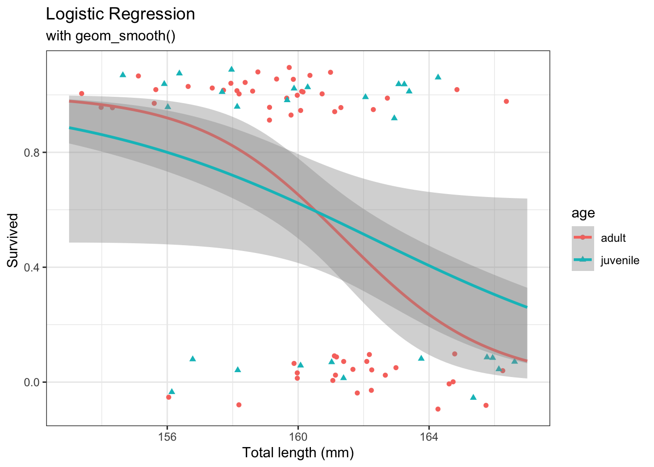
This chapter introduced logistic regression for a single binary response variable with up to two explanatory variables. The focus of this chapter has been on our ability visualize model fits using ggplot graphics with either geom_smooth or manually creating lines using predict and geom_line.